Experiment 10: Measuring a Human Hair

Objective:
To determine the thickness of a human hair using two methods. Measurement through laser diffraction and direct measurement using a micrometer.

Equipment:
-Laser
-Paper (hole punched)
-Micrometer
-Strand of hair
-Meter stick or ruler
-Clamps

Procedure:

For the first part of the lab, we had to turn on the laser and observe the diffraction pattern that resulted on a screen at a set distance.

We then marked the pattern on the whiteboard so we could do the calculations.

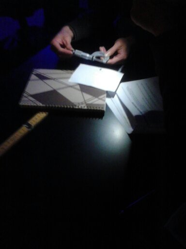
For the second part of the lab, we used a micrometer to obtain a value for the thickness of a human hair.

Data/Calculations:

Using the formula y = λL/d for the interference between two slits, we obtained L by measuring the distance from the system to the screen and λ by noting the given wavelength of the laser. We obtained y by measuring the total distance five constructive interference strips (in millimeters) generated and divided this number by five to obtain y, the distance from the first constructive interference maximum (red strip) from the center strip.

For the second part of the experiment, we each took turns measuring the diameter of the hair using the micrometer and we averaged out our values.


We obtained the results on the table below:

Conclusion:
Our results where considerably accurate when we calculated the diameter using the diffraction method, however, the measurements with the micrometer where a lot more accurate than this because this is the micrometer's primary function, therefore, it should be considered closer to the true value. The diffraction method is a lot less accurate because there is a significantly larger source for error in measurements, also, the situation is not an idealized two infinitesimally-small slit interference pattern.

Experiment 9: Lenses

Objective:
To observe the characteristics of converging lenses by placing an object on one side of said lens and observing the real, inverted image that is created on the other of the lens.

Equipment;

-Light box
-Converging lens
-Lens holder
-Meter stick
-Index card (or anything else to project the image on)

Procedure:

We determined the focus by having two lasers go through the lens and moving the board onto which they were projected around until they converged into one dot. The distance from this board to the lens was the focus.

For the second part of this experiment, we measured how the object distance affected the image distance and image height and recorded our results on a table. We varied the object distance by moving the lens further away and we obtained an image height by varying the position of the paper the image was projected upon until we could see a clear image.

Lastly, we evaluated what happened to the image when the object distance was at 0.5 f, we concluded that the image went to infinity (diverged).

Data/Calculations:
The table below shows the data we gathered:

We first plotted the image distance vs. the object distance and found that it possessed an inverse relationship:

By plotting the inverse of the image distance vs. the negative inverse of the object distance, we obtain a linear relationship that can be explained by the equation 1/s + 1/s' = 1/f.

Conclusion:
After plotting the inverse values and noticing that the graph is linear, it can be concluded that it is of the form y=mx + b. Substituting what y and x are the equation 1/q = -m/p + b. Comparing it to the standard 1/s + 1/s' = 1/f equation relating object distance s and image distance s' it makes sense that m is equal to 1 and b is equal to 1/f, we obtained a slope of .9 and a y intercept of .184 so we were very close to the actual values. This experiment proves that the object and image distance relationship works. There were some inaccuracies in our experiment and they were accounted for with uncertainties since it was very difficult to get accurate measurements.

Experiment 8: Concave and Convex Mirrors

Introduction:
In this experiment we observed the images created by concave and convex mirrors.

Equipment:
-Convex Mirror
-Concave Mirror
-Object/person

Experiment:
Part A: Convex Mirror

1. Images reflected on convex mirrors had the following characteristics:
-smaller than the original object
-upright
-looked closer relative to the position of mirror and object.

2. As you moved closer, nothing really changed other than the image getting a bit larger due to the fact you were closer to it.

3. The image becomes significantly smaller as you move far away.
Part B: Concave Mirror

1. Objects closer to this type of mirror created images with the following characteristics:
-Image appeared larger than the original object
-The image was upright
-It looked closer than the original object.

2. As you moved closer to the mirror, the image became very distorted and significantly bigger.

3. Distant objects created images with the following characteristics:

-Image appeared smaller than the original object
-The image was inverted
-It looks closer relative to the position of image and object

Data/Calculations:
Part A: Convex Mirror

Part B: Concave Mirror

Conclusion:
Images formed by concave mirrors can vary from being very large and upright to small and inverted while convex mirrors create images that are magnified and remain upright. This is probably due to the fact that the focus is only approachable in the case of the concave mirror.

Experiment 7: Introduction to Reflection and Refraction

Introduction:
This experiment allows us to observe the effects light traveling from mediums of different densities.

Equipment:

-Light box
-Semicircular plastic/glass prism
-Circular protractor

Procedure:
There were two parts to this experiment. The first consisted of having the flat side of the semicircular prism face the light ray and treat this as an incidence from the air to the glass. In the second part of this experiment, the circular side of the prism was facing the light ray, and we treated this as incidence from the class to the air.

Part 1:

Prior to starting the observations, we made some initial predictions of what would occur, mainly that for the original incidence there would be a zero angle of refraction (perpendicular to normal between both mediums) and that at other incident angles there would be angles of refraction because the densities of both mediums varied. In this first part of the experiment, the light is traveling from the lower density medium (air) to glass. Which means the angle of refraction (respect to the normal) should be less than the incident angle according to Snell's Law.

Part 2:

Similar to the first part, we had to make some initial predictions before starting the experiment. Like the first part of the experiment, the incident angle will equal the refracted angle if the angle of incidence is zero with respect to the normal between the two mediums. This case involves light traveling from a higher density material (glass) to the less dense air. According to Snell's Law, the angle of refraction should be greater than the angle of incidence.

Data/Calculations:
Part1:
Below is a table of the information we gathered for the first part of the experiment.

The following is a graph of theta one versus theta two. It appears you can fit a simple line equation in the order of y = mx + b to it.

The graph below is that of sin theta one versus sin theta two. The regression line for the graph is shown. The slope of this graph is about 1.5, according to Snell's Law, this should be equal to the index of refraction of the glass. The relationship in this straight line deals with how strongly the light will be bent upon reaching a medium with a greater index of refraction.

Part 2:

Similarly, we gather information and record these results on a table.

We had to do certain angles instead of the ones we had planned to (else we wouldn't have gotten ten cases) because we reached the critical angle where none of the light was refracted.

Like the first part, we graph sin theta 2 versus sin theta 1 and linear fit this. The slope of this line is one, and judging from Snell's Law, this represents air's index of refraction. This is not the same as the equation we found previously because the beam of light traversed the glass before the air in part 2.

Summary:
This lab went quite smoothly even though there were a few sources of error such as not being able to measure angles with ideal precision. Upon looking at the actual index of refraction for these materials, we can see that our experimental values came pretty close.

Experiment 6: Electromagnetic Radiation

Introduction:
We observe the phenomena of electromagnetic waves from a transmitting antenna to a receiver.

Equipment:

-Oscilloscope
-Oscillator
-BNC adapter (point receiver)
-Copper wire (antenna)
-Meter stick

Procedure:

On the oscillator we dialed a frequency of 30kHZ. We changed the time/division on the oscillascope and the voltage/division until we could see a signal on the screen.
To verify that the signal we saw on the oscilloscope was generated by the antenna we performed the following tests:
1. Moving the antenna closer made the wave amplitude larger.
2. Moving the antenna farther made the wave amplitude smaller.
3. Not moving the antenna kept the wave amplitude the same.

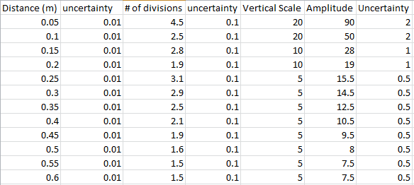
We then proceeded to measure the amplitudes at certain equal intervals of distance from the receiving antenna to observe how the wave amplitude varied across this range.

Data/Calculations:
Below is a table containing the data we gathered in this experiment.

Below is a graph of the peak-to-peak amplitude as a function of distance. This scatter plot seems hyperbolic in nature.

Trig Variant:
The first graph is the data fitted with the function A/R while the second one fits the data with A/R^2. The first graph appears to fit the data most accurately.

The final graph below is a fit with the function A/R^n. This fit seems to be on par with a fit of A/R.

Summary:
We would expect 1/r to fit well if the transmitter were a point charge, but because this is simply not true (our transmitter was a copper wire with a certain length). This

Experiment 5: Introduction to Sound

Introduction:

In this experiment we observe and measure various properties of sound waves.

Equipment:

-Loggerpro

-Microphone

-Tuning fork

Procedure:

Two of us tried our best to say "AAAAAAAA" smoothly into the microphone, in the third section of this experiment, we had to use a tuning fork instead. The sound waves were recorded by loggerpro and we got to observe a graphic representation of the waves to calculate some of their various qualities.

Data/Calculations:

Graph for part 1:

Graph for Part 2:

Graph for Part 3:

Graph for Part 4:

Summary:

It was rather difficult to get any decent looking waves in this experiment, especially using our voices because even the most minimal alteration during the process would most likely cause the wave to change.

Experiment 4: Standing Waves

Introduction:
We generated various normal modes and analyzed the various resonant conditions for standing waves on a string.

Equipment:

-Pasco variable frequency wave driver
-String
-Pasco student function generator
-Weight set (grams)
-Pendulim clamp
-Pulley
-Digital Multimeter
-Meter stick

Procedure:

We took some initial measurements (mass and length of the string) and we set up the system. We then took various measurements for different harmonics (such as number of nodes, antinodes, wavelength) and we achieved such harmonics by adjusting the frequency of the function generator. This was done for two instances, the second of which was equivalent to one-fourth the original tension.

Data/Calculations:

We went through ten harmonics in case one and six in case two by toggling with the frequency generator. We recorded the frequencies that produced such harmonics and length from one node to another to calculate the wavelength. We also counted the number of nodes and anti-nodes and recorded them on the table above.

Above are the graphs we created by plotting the frequency versus one over the wavelength, the graph's slope should equal the wave speed.

We calculated the experimental values for their respective velocities using the formula shown above.

Above are the wave speeds from the graph and the wave speeds we calculated respectively. The experimental and theoretical values both seem to vary by a factor of two.

We can see from the table above that the experimental value of frequencies is around n times the frequency of the fundamental. Where n is the number of the harmonic.

The table above is obtained from taking the ratios between the frequencies in the first case and the ones in the second case. They also seem to differ by a factor of two.
Summary:
This experiment was surprisingly very accurate when comparing the values obtained from formulas and the values obtained from our observations. There are many factors that make them differ, however, such as wind resistance and the fact that we where conducting this experiment in a three dimensional space (the string not only oscillated, but also sort of spun in circles).